
When I wrote about training a Transformer from scratch, I focused on the engineering chain: preparing data, choosing a tokenizer, saving a model, and understanding why low loss did not guarantee useful answers. Reading Karpathy's MicroGPT made me want to go one level deeper.
If I remove MLX, PyTorch, tensor operations, and the GPU, what remains of GPT training?
My answer is a function that assigns probabilities to the next token, a graph that records how its calculations depend on one another, and a rule for changing parameters in response to error. At this scale, I can trace an individual multiplication all the way to an output probability.
This article uses source snapshot 14fb038 as its reference. The derivations, worked examples, and diagrams below are my explanation. The numerical examples illustrate calculations; they are not training results. A name generator also should not be mistaken for a general language assistant.
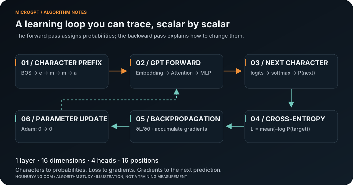
Start with the prediction task
Take one training example, emma. The model learns a sequence of conditional probabilities:
P(emma, END | START)
= P(e | START)
× P(m | START,e)
× P(m | START,e,m)
× P(a | START,e,m,m)
× P(END | START,e,m,m,a)
This is the probability chain rule applied to a sequence. GPT implements each conditional distribution with the same parameters. Different prefixes produce different probabilities.
In this implementation, characters map to integer IDs, and the special token BOS appears at both ends. START and END in the explanation therefore share one ID. The model learns both how to begin and when to stop.
| Position | Current input | Visible prefix | Target |
|---|---|---|---|
| 0 | BOS | BOS | e |
| 1 | e | BOS e | m |
| 2 | m | BOS e m | m |
| 3 | m | BOS e m m | a |
| 4 | a | BOS e m m a | BOS |
The target shifts one position ahead, and attention can only use current and earlier inputs. Both conditions are necessary. Without the shift, a model could learn to copy. With access to future inputs, it could inspect the answer.
During training, the next input is the real character from the data: teacher forcing. Even if the model guesses the wrong character, the following position still receives the correct one. During generation, the next input is the model's own sample. A mistake then changes the prefix used for every subsequent prediction.
How does a parameter know which way to move?
For me, the best entry into MicroGPT is a multiplication node, before attention enters the picture.
Let a = 2, b = 3, u = a × b, and L = u + a. The forward result is 8. Backward computation asks how much L would change if a or b changed slightly:
∂L/∂u = 1
∂u/∂a = b = 3
∂u/∂b = a = 2

∂L/∂a = (∂L/∂u)(∂u/∂a) + 1 = 4
∂L/∂b = (∂L/∂u)(∂u/∂b)     = 2
There are two paths from a to L. Their contributions must add. Replacing gradient accumulation with assignment silently loses a path.
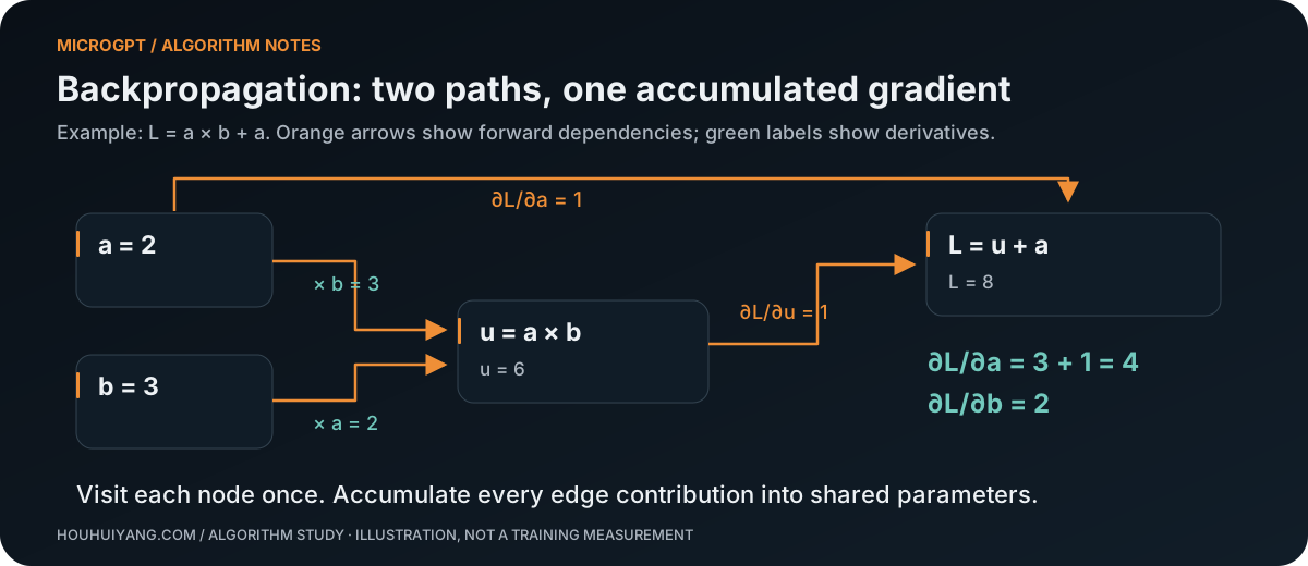
An automatic differentiation scalar needs four kinds of information: its current value, its accumulated gradient, its input nodes, and its local derivatives with respect to those inputs. Forward operations record dependencies. Backward operations propagate gradients through them.
| Local operation | Local derivative |
|---|---|
z = a + b | 1 for each input |
z = a × b | b with respect to a; a with respect to b |
z = a^k | k × a^(k−1), for constant k |
z = log(a) | 1/a |
z = exp(a) | exp(a) |
z = ReLU(a) | 1 above zero, 0 below; choose 0 at zero |
These rules compose into linear layers, normalization, softmax, and loss. A matrix is a container of scalars; its multiplication can be expressed as individual products and sums.
Backward propagation runs in reverse topological order. A node must collect all contributions from operations that consume it before passing the accumulated result to its inputs. Set ∂L/∂L = 1, then apply:
input gradient += output gradient × local derivative along this edge
Deduplicate nodes when ordering the graph, but preserve repeated input edges. In a × a, both edges contribute, producing 2a.
Parameter sharing follows the same rule. One embedding row can participate at multiple positions. It remains one set of parameter objects, and gradients from those positions accumulate into them.
Account for every parameter
The reference configuration has one layer, hidden width 16, four heads, and 16 context positions. Each head has width 4; the MLP expands to width 64. Let V be the vocabulary size. Matrices are stored as output width by input width.
| Parameters | Shape | Count |
|---|---|---|
| Token embedding | V × 16 | 16V |
| Position embedding | 16 × 16 | 256 |
| Q, K, V, O projections | 16 × 16 each | 1,024 |
| First MLP projection | 64 × 16 | 1,024 |
| Second MLP projection | 16 × 64 | 1,024 |
| Output LM head | V × 16 | 16V |
| Total | No biases or learned normalization gains | 32V + 3,328 |
For 26 letters plus BOS, V = 27 and the total is 4,192 parameters. This is a calculation from the shapes, not a constant for every custom dataset. The token embedding and output head are separate matrices in this version; their weights are not tied.
An integer token ID is an address, not a semantic coordinate. Character 20 is not inherently twice character 10. The ID selects a learned vector. Adding a learned position vector lets the representation distinguish where the character occurs.
Follow one forward pass
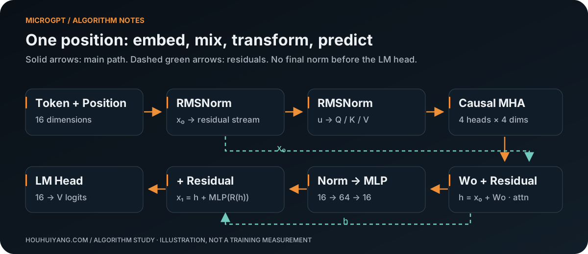
I use column vectors for a single position to keep the data flow visible. Let R denote RMSNorm, E the token embedding table, and P the position table:
x₀ = R(E[token] + P[position])

u = R(x₀)
q = Wq u,  k = Wk u,  v = Wv u
h = x₀ + Wo · MultiHeadAttention(q, K≤t, V≤t)

r = R(h)
x₁ = h + W₂ · ReLU(W₁ r)

logits = Wout x₁
probabilities = softmax(logits)
This describes the one-layer implementation. Do not silently insert a final normalization: this snapshot sends the last residual output directly to the LM head. It is a simplified decoder-only model, not an exact GPT-2 reproduction.
RMSNorm controls the scale
For a vector with d elements:
mean_square = (x₁² + ... + x_d²) / d
R(xᵢ) = xᵢ / sqrt(mean_square + ε)
For [3, 4], ignoring the small epsilon, the denominator is sqrt(12.5) and the result is approximately [0.8485, 1.1314]. This does not subtract the mean or make all elements identical. It adjusts the overall scale while preserving direction.
MicroGPT's variant omits a learned gain vector and uses epsilon 1e-5.
Two normalizations appear near the beginning, which can look redundant. But the first normalized vector also enters the residual path; the second normalization belongs only to the attention branch. Similar forward values do not justify removing the first operation: that changes the residual stream and its gradient path.
Residuals let a block learn a correction
For y = x + F(x), the derivative includes a direct path: ∂y/∂x = I + ∂F/∂x. Existing information can survive while a block adds a correction. This helps gradient propagation, but does not guarantee stable training at arbitrary depth or learning rate.
What attention actually computes
I think of Q, K, and V as three roles. Q determines how the current position searches for information. K determines how a visible position participates in matching. V carries the content to be combined. These are learned projections, not fields with meanings assigned by the programmer.
For position t in one head:
score(t,j) = dot(q_t, k_j) / sqrt(d_head)     j ≤ t
weight(t,j) = exp(score(t,j)) / Σ exp(score(t,r))
output_t = Σ weight(t,j) × v_j
The normalization and weighted sum run only over visible positions. Four heads each return four numbers. Concatenating them gives 16 numbers, followed by an output projection. This applies scaled dot-product and multi-head attention at a very small width.
Why divide by the square root of head width? Under idealized assumptions of independent, zero-mean components with suitable variance, dot-product variance grows with dimension. Scaling helps prevent dimension alone from pushing softmax toward overly sharp distributions. With head width 4, the divisor is 2, not 4 or 16.
Here is a constructed example. Use q = [1, 0, 1, 0] and three visible keys: [1, 0, 0, 0], [0, 1, 0, 0], and [1, 0, 1, 0]:
Dot products     = [1, 0, 2]
Scaled scores    = [0.5, 0, 1]
Softmax weights  ≈ [0.3072, 0.1863, 0.5065]

For values:
[1, 0, 0, 0], [0, 2, 0, 0], [0, 0, 3, 0]
The output is approximately:
[0.3072, 0.3726, 1.5194, 0]
Attention blends information instead of selecting just one position. Its weights are also not output-token probabilities. Attention normalizes over visible positions; the language-model output normalizes over vocabulary entries. Projections, residuals, and an MLP sit between them.
Causality without an explicit mask
A parallel implementation usually constructs scores for all position pairs, then assigns negative infinity to future positions so their softmax weights become zero. MicroGPT advances one position at a time. It computes the current K and V, appends them to the current layer's lists, and attends only to entries already present.
At position t, those lists contain positions 0...t. Future information is absent from the accessible data structure. Execution order enforces causality.
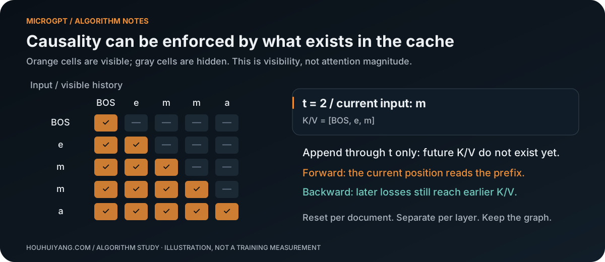
During training, these K/V entries remain attached to the computation graph. A later position's loss can propagate through attention into earlier K/V projections and embeddings. Preventing forward access to future inputs does not prevent a later loss from sending gradients to earlier computations.
Each document or generated sample needs fresh lists, and each layer needs its own lists. At inference, historical K/V can be cached as values without gradients. Detaching them during training would cut required gradient paths.
This is not an automatically sliding, unlimited context window. There are only 16 learned position rows. Training uses at most the first 16 prediction positions, and generation runs at most 16 iterations. Longer custom documents do not automatically become multiple windows. They need an explicit slicing policy; otherwise even the closing boundary token may be excluded from training.
Connect the MLP, softmax, and loss
Attention mixes information across positions. The MLP applies a nonlinear transformation to each position's representation: 16 dimensions to 64, ReLU, then back to 16.
Without a nonlinearity, two linear transformations collapse into one: W₂(W₁x) = (W₂W₁)x. ReLU prevents that general collapse and allows different feature combinations to activate for different inputs.
The LM head produces one logit per vocabulary entry. Logits can be negative and need not sum to one. Softmax turns them into probabilities:
pᵢ = exp(zᵢ − c) / Σⱼ exp(zⱼ − c)
c = max(z)
Subtracting a common constant leaves the probabilities unchanged because the common factor cancels. Choosing the maximum prevents large positive exponential arguments. Treating c as an ordinary number preserves the correct derivative here because softmax is invariant to a shared shift. Extremely small probabilities can still underflow; production training typically uses a stable log-softmax or fused cross-entropy rather than computing tiny probabilities and then taking their logarithm.
For target y, the position loss is L_t = −log(p_y). Raising the correct token's probability from 0.1 to 0.5 lowers loss from about 2.3026 to 0.6931. The document loss averages all valid prediction positions, not just the final character.
The derivative is particularly useful. Starting from L = −z_y + log(Σ exp(z_j)), differentiation gives:
∂L/∂zᵢ = pᵢ − 1[i = y]
For predicted probabilities [0.2, 0.5, 0.3] with the first entry correct, the logit gradient is [-0.8, 0.5, 0.3]. Gradient descent directly raises the correct logit and lowers the others. The chain rule carries that signal back to the contributing parameters. Averaging over n positions divides each position's contribution by n.
Uniform guessing over 27 classes gives ln(27) ≈ 3.2958 loss and perplexity 27. That is a theoretical reference, not an exact prediction of the first printed loss: random initialization need not produce a perfectly uniform distribution.
How Adam turns gradients into updates
Plain gradient descent uses θ ← θ − ηg. Adam additionally maintains exponential moving averages of gradients and squared gradients, adapting update scales per parameter. The update can be expanded directly.
Let s count optimizer steps starting at 1, separately from token positions:
m_s = β₁ m_(s−1) + (1−β₁) g_s
v_s = β₂ v_(s−1) + (1−β₂) g_s²

m̂_s = m_s / (1−β₁^s)
v̂_s = v_s / (1−β₂^s)

θ_s = θ_(s−1) − η_s × m̂_s / (sqrt(v̂_s) + ε)
Bias correction compensates for moments initialized to zero. The source uses beta values 0.85 and 0.99, initial learning rate 0.01, and linear learning-rate decay. This is Adam, without AdamW's decoupled weight decay.
For a first gradient of 0.2, m becomes 0.03 and v becomes 0.0004. Their corrected values are 0.2 and 0.04. Ignoring the tiny epsilon, the first update subtracts approximately 0.01. A larger raw gradient therefore does not automatically imply a proportionally larger Adam step.
The training loop can be expressed independently as the following pseudocode. It is a reading aid, not a runnable GPT implementation:
Initialize parameters θ and Adam state m, v
For each step:
    Select one document, encode it, and add boundary markers
    Create fresh K/V lists for every layer
    Compute next-token losses using the real prefix at each valid position
    Average the losses and backpropagate once
    Update θ with Adam and clear parameter gradients
Averaging each document before one update makes the document the sampling unit. This is not automatically equivalent to averaging every token in the entire corpus: document length changes the relative weight of an individual token.
The default 1,000 steps are not 1,000 epochs. A step processes one document; an epoch requires a full pass through the dataset. The decay formula also uses a zero-based step index, so the last update has a small positive learning rate rather than exactly zero.
During generation, learning has stopped
Start with BOS, compute logits, apply temperature, sample a token, and feed it into the next position. Stop on BOS or after at most 16 generated characters.
pᵢ(T) = exp(zᵢ / T) / Σⱼ exp(zⱼ / T) T > 0
For two logits separated by 1, the probability ratio is approximately 2.72 at T = 1 and 7.39 at T = 0.5. Lower temperature concentrates the distribution. It does not add knowledge or guarantee factual correctness. Temperatures above 1 are valid; zero cannot be inserted into this division and normally requires a separate greedy-selection path.
Inference performs no loss backward pass or Adam update. Reading the prefix changes activations and cache contents, not long-term parameters. This minimal implementation reuses autograd operations, so it still incurs graph-building overhead. Omitting backward is not equivalent to implementing a framework's no-grad mode.
A plausible name suggests that some character regularities were learned. Novel-looking output alone does not establish that the model avoided memorization. Generalization needs held-out examples, overlap checks, and evaluation aligned with the intended task.
How I would verify an implementation
Short code can still be wrong. I would start with calculations I can check by hand, then look at training curves.
- Shared-node gradients:
L = a×b+aat a=2, b=3 must yield gradients 4 and 2.a×amust yield2a. - Numerical gradients: compare selected automatic derivatives with central differences,
(L(θ+h)−L(θ−h))/(2h), avoiding ReLU's kink at zero. - Causality: changing a suffix while keeping the prefix fixed must leave prefix logits unchanged. A parallel rewrite should also agree with the sequential version.
- Loss and updates: check probability normalization, cross-entropy derivatives, the first Adam update, and gradient clearing after every step.
- Data boundaries: verify BOS pairing, truncation, and vocabulary coverage before trying tiny-set overfitting and independent validation.
I prepared a dependency-free calculation check for this article. It covers shared-node backpropagation, central differences, the attention example, cross-entropy gradients, and the first Adam update. It checks the mathematical examples, not complete GPT training or performance.
To run the author's implementation, save the pinned source as microgpt.py in a separate empty directory and execute python3 microgpt.py. If input.txt is absent, the script downloads the default names dataset. A custom file should contain one nonempty example per line; keep the character vocabulary and 16-position truncation in mind. The current Gist and its revisions can be compared with the pinned version.
What a complete algorithm means to me
MicroGPT connects ideas that are often learned separately into one traceable path. Characters select input vectors. Attention mixes context. The output layer assigns probabilities. Loss produces gradients. The optimizer changes parameters. Those changes affect the next prediction.
Reaching a useful language model still requires decisions about data quality, tokenization, architecture, training objectives, evaluation, and post-training. These cannot all be reduced to execution speed. GPUs, batching, and fused kernels primarily change how efficiently computation runs. Different data and supervision change what the model learns.
For my own engineering work, the code suggests a practical debugging order. Wrong predictions: inspect target alignment. No learning: inspect gradient paths. Suspiciously good loss: check for future leakage. Strange samples: inspect probability conversion and stopping conditions.
This is the level of understanding I want to keep: relationships I can inspect. Knowing where a number came from gives me a reasoned way to decide what to change next.